I intend to explain a very powerful concept in data conversion: the Sigma-Delta loop. Before I do so, I will describe quantization noise (which sigma delta loops attempt to alleviate).
Quantization noise occurs during the analog-to-digital conversion (ADC) process. Since an analog signal can attain any value, it has infinite precision. This infinite precision excludes the fact that all analog signals have some amount of circuit noise that limits their precision. On the other hand, digital signals are represented as 0s and 1s—and a finite combination of them. As a result, during the conversion, we go from an infinite precision to a finite precision. The resulting error in this rounding is called quantization noise.
We will analyze 3 examples of quantization, and analyze the noise both in the time domain and in the frequency domain.
Sampled Sinusoid
Our first example of quantization is that of an infinitely precise sinusoid. In this case, we are sampling this sinusoid at 16x its frequency. The sinusoid frequency is 1/16 Hz. The sampling rate is 1 Hz. So, for every cycle of the sinusoid, we get 16 samples:
| time | sin(2*pi*t/16) | Rounded (4-bit) | Error |
| 0 | 0.00000 | 0.000 | 0.00000 |
| 1 | 0.38268 | 0.375 | -0.00768 |
| 2 | 0.70711 | 0.750 | 0.04289 |
| 3 | 0.92388 | 0.875 | -0.04888 |
| 4 | 1.00000 | 1.000 | 0.00000 |
| 5 | 0.92388 | 0.875 | -0.04888 |
| 6 | 0.70711 | 0.750 | 0.04289 |
| 7 | 0.38268 | 0.375 | -0.00768 |
| 8 | 0.00000 | 0.000 | 0.00000 |
| 9 | -0.38268 | -0.375 | 0.00768 |
| 10 | -0.70711 | -0.750 | -0.04289 |
| 11 | -0.92388 | -0.875 | 0.04888 |
| 12 | -1.00000 | -1.000 | 0.00000 |
| 13 | -0.92388 | -0.875 | 0.04888 |
| 14 | -0.70711 | -0.750 | -0.04289 |
| 15 | -0.38268 | -0.375 | 0.00768 |
| 16 | 0.00000 | 0.000 | 0.00000 |
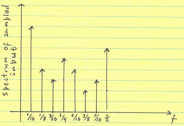
The important thing to note is that the error (since it is solely dependent on the sinusoid) is periodic. It repeats every 16 samples. (In fact, it inverts itself every 8 samples.)
This periodicity results in tones of the sinusoid in the spectral analysis of the samples:
Sum of Four Prime Sinusoids
In this case, we sum 4 sinusoids, of frequency 1/15 Hz, 1/16 Hz, 1/17 Hz, and 1/19 Hz.
| Time | (sin(2*pi*t/15)+sin(2*pi*t/16)+sin(2*pi*t/17)+sin(2*pi*t/19))/4 | Rounding (4-bit) | Error |
| 0 | 0.00000 | 0.000 | 0.00000 |
| 1 | 0.36884 | 0.375 | 0.00616 |
| 2 | 0.68454 | 0.625 | -0.05954 |
| 3 | 0.90182 | 0.875 | -0.02682 |
| 4 | 0.98991 | 1.000 | 0.01009 |
| 5 | 0.93708 | 0.875 | -0.06208 |
| 6 | 0.75217 | 0.750 | -0.00217 |
| 7 | 0.46319 | 0.500 | 0.03681 |
| 8 | 0.11295 | 0.125 | 0.01205 |
| 9 | -0.24741 | -0.250 | -0.00259 |
| 10 | -0.56604 | -0.625 | -0.05896 |
| 11 | -0.79809 | -0.750 | 0.04809 |
| 12 | -0.91215 | -0.875 | 0.03715 |
| 13 | -0.89463 | -0.875 | 0.01963 |
| 14 | -0.75140 | -0.750 | 0.00140 |
| 15 | -0.50644 | -0.500 | 0.00644 |
| 16 | -0.19792 | -0.250 | -0.05208 |
| 17 | 0.12790 | 0.125 | -0.00290 |
| 18 | 0.42368 | 0.375 | -0.04868 |
| 19 | 0.64802 | 0.625 | -0.02302 |
| 20 | 0.77147 | 0.750 | -0.02147 |
| 21 | 0.78040 | 0.750 | -0.03040 |
| 22 | 0.67850 | 0.625 | -0.05350 |
| 23 | 0.48555 | 0.500 | 0.01445 |
| 24 | 0.23381 | 0.250 | 0.01619 |
| 25 | -0.03730 | 0.000 | 0.03730 |
| 26 | -0.28741 | -0.250 | 0.03741 |
| 27 | -0.48136 | -0.500 | -0.01864 |
| 28 | -0.59414 | -0.625 | -0.03086 |
You’ll notice that in this case, the quantization error does not repeat. It will repeat eventually (after 77520 samples)—because that is when the input repeats. In our little observation window, things look random. The point of this example is that depending on the complexity of the input, the quantization noise can look random:
We don’t merely see harmonics of each input—we see complex inter-modulations of these tones. I dislike the term inter-modulation in this case since there are really no polynomial non-linearities in the quantizer. In fact, one cannot see any pattern to the resulting non-linearities: they are not stronger near the harmonics of the tones, exhibiting trailing side-bands that are characteristic of true inter-modulation.
In fact, I often wonder as a circuit designer if our methods of applying a sinusoid and computing noise and distortion are overly conservative. Agreed, they give us insight in the workings of the circuits. But, do they accurately predict the behavior of the system for (say) CDMA or OFDM modulation on it? What if we add a GSM or VSB adjacent channel?
Sinusoid with Random Noise
Our final case is a sinusoidal input (such as in the first example) with added random noise to it.
| time | sin(2*pi*t/16)+noise | Rounded (4-bit) | Error |
| 0 | 0.15839 | 0.125 | -0.03339 |
| 1 | 0.51863 | 0.500 | -0.01863 |
| 2 | 0.76647 | 0.750 | -0.01647 |
| 3 | 1.10245 | 1.125 | 0.02255 |
| 4 | 1.07941 | 1.125 | 0.04559 |
| 5 | 1.04485 | 1.000 | -0.04485 |
| 6 | 0.81284 | 0.875 | 0.06216 |
| 7 | 0.48070 | 0.500 | 0.01930 |
| 8 | 0.15675 | 0.125 | -0.03175 |
| 9 | -0.23475 | -0.250 | -0.01525 |
| 10 | -0.55725 | -0.500 | 0.05725 |
| 11 | -0.83914 | -0.875 | -0.03586 |
| 12 | -0.84315 | -0.875 | -0.03185 |
| 13 | -0.80978 | -0.750 | 0.05978 |
| 14 | -0.69691 | -0.750 | -0.05309 |
| 15 | -0.33005 | -0.375 | -0.04495 |
| 16 | 0.13032 | 0.125 | -0.00532 |
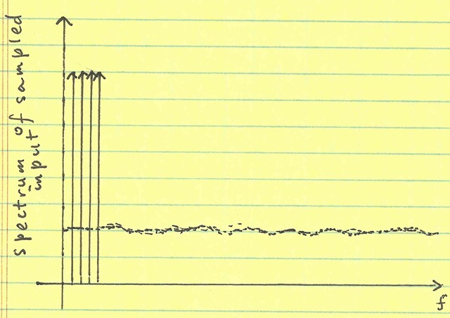
I have chosen the noise to be large enough to overwhelm the input. In this case, the error no longer looks periodic. Its statistics are basically dictated by the noise, not the signal.
In this case, there is no tonal quality to the quantization noise—not even over large periods of observation (in contrast to the previous example). In fact, this method of adding noise (called dither) is often used in audio equipment, since audiophiles have a larger aversion to tonal distortion than to random noise.
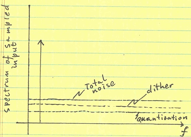
There’s no free lunch here. The overall spectrum exhibits more total error (the added dither plus the quantization noise) than in the first example—we have improved the quality of the overall noise, but not the quantity:
In contrast, the sigma-delta loop randomizes noise by introducing a chaotic memory element. I will explain the sigma-delta in detail in the future posts.
[…] Circuit Design Tutorials and Insights in Electronics and Circuit Design Skip to content About « Quantization […]