I’ve been doing some statistical measurements lately (more to follow). It occurs to me that while most people measure the mean of a set of measurements, the median is more useful.
If the distribution is Gaussian, the mean and median are equal.
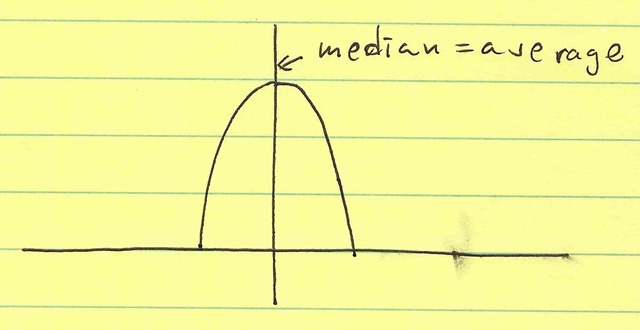
(Mean is defined as $\mu_X = \int X p(X) dX$ where $p(X)$ is the probability distribution function (PDF) of $X$—that is, it’s a average of X, weighted with the probability density of $X$. The median defined as $P ( X < \mu_{1/2} ) = 1/2$—that is, the point where $X$ is equally likely to be lower than or greater than (50% probability).)
Many times in engineering and process control, we keep track of the mean and standard deviation. One of the reasons is that if the thing we’re trying to control is Gaussian, the mean/median and standard deviation give us good design criteria to minimize failure: if we allow our system to tolerate $\pm 3$ standard deviations ($6 \sigma$) around the mean/median, then it has a 99.7% chance of success (0.3% chance of failure).
However, we can generalize this: if we wanted to be more lax, we could only design (or require) the system to tolerate $\pm 2$ standard deviations (4.5% failure). In some cases, systems are designed to tolerate $\pm 4$ standard deviations (0.006% failure). So, one can design the system to tolerate $\mu_(1/2) \pm k \sigma$, where $k$ is some factor (3, 2, 4 for example) that determines the probability of failure.
However, what if the distribution is bimodal? Take for example, two modes of operation (each more or less Gaussian):
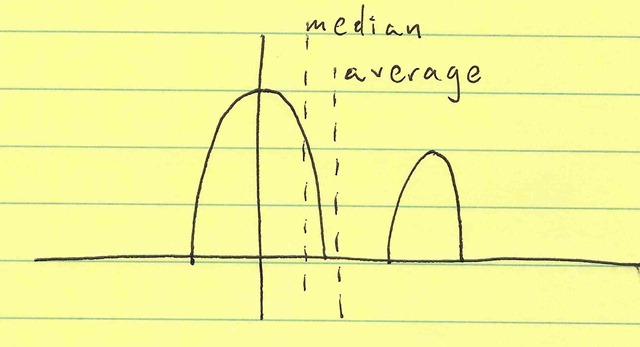
Due to the asymmetric distribution, the mean and median are now not the same. In this case, we could posit that some secondary mode (or external factor) causes that second hump. Let’s call the main hump the primary mode and the smaller hump the secondary mode. If things are behaving “normally” we get the first hump, but some failure or aberration causes the second hump.
However, what if the system was more sensitive to this failure (secondary mode). Then, we’d see something like: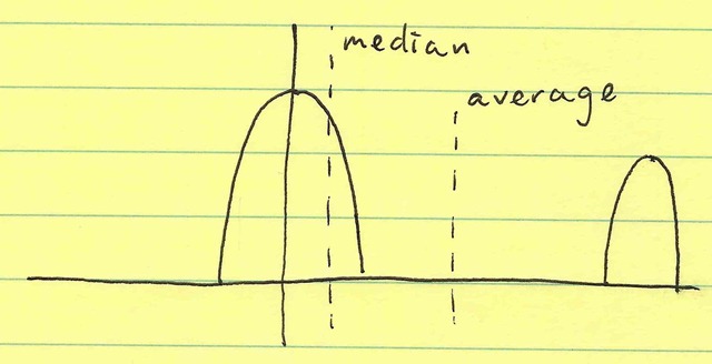 Notice what happened? The median stayed exactly the same. However the mean mislabeled “average”) moved proportionally to that secondary hump. Incidentally, the standard deviation ($\sigma$) also moved proportionally to the distance between the two humps—but let’s focus on the fact that the mean just changed.
The question you’re probably asking is “what’s so bad about that”? Well, if you’re computing six-sigma-like design criteria, you’re taking $\mu \pm k \sigma$. Recall, however, that we could pick any factor $k$ depending on the probability of failure we want (I should say want to avoid). So, when both the average and the standard deviation change, how can we be sure we’re getting the right value for $\mu + k \sigma$?
The nice thing about picking the median as the average is that it doesn’t depend on the magnitude of the secondary mode—only on the probability of the secondary mode. The magnitude of failure impacts the standard deviation. I like to view these (median and standard deviation) as two independent metrics that tell different stories.
Another thing to note is that one could view the 2nd illustration above as an input to a nonlinear amplifier (for example) and the 3rd illustration as the output. That’s another nice thing about the median: it commutes with a monotonic nonlinearity. That is, if $f$ is monotonic, and $Y = f(X)$, then $\mu_{1/2,Y} = f(\mu_{1/2,X})$. So, we don’t have to worry so much that we’re measuring the correct independent variable. Our median will give us the same information (albeit in a different, nonlinear domain).